Embedded 101: MicroPython Performance Optimization — Steps & Practical Cases from Slow to Fast
This article details MicroPython performance optimizations such as memory tuning, native/viper compilation, mpy-cross and RP2040 hardware optimizations.
COMPONENTS
PROJECT DESCRIPTION
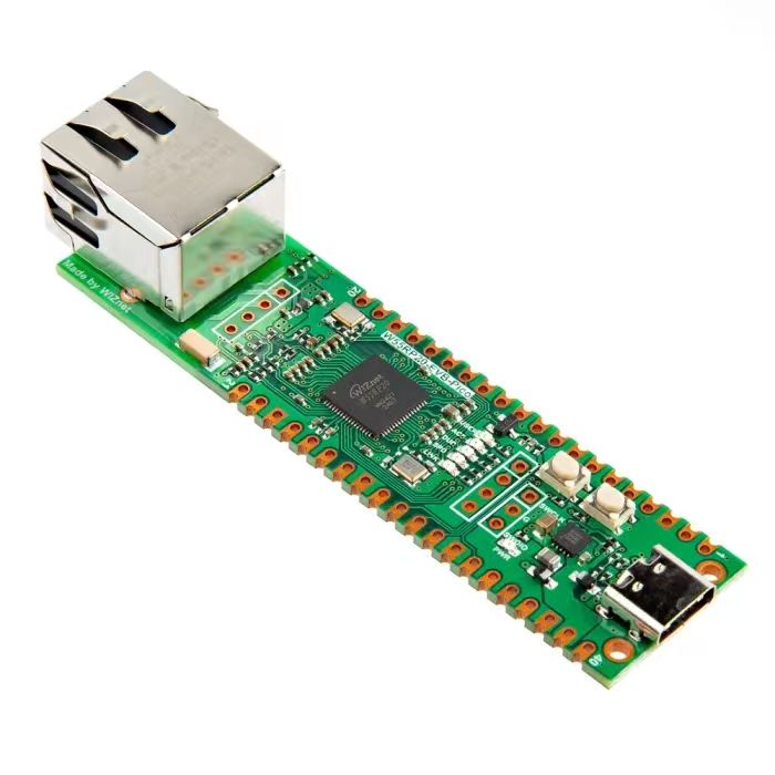
【Preliminary Note】The original hardware example in this article was written based on the RP2040. The actual hardware used in this hands-on demonstration features the W55RP20 as the main controller chip. The circuit logic and UF2 flashing operation principles are universally applicable, with only the main controller model differing. The original chip model mentioned in the circuit descriptions below is provided for reference purposes only.
1. Maximize the running speed of MicroPython
Optimization Idea: Optimize in the order of "from simple to complex, from software to hardware", first identify the performance bottleneck, then make gradual adjustments to achieve the maximum performance improvement at the lowest cost.
The core tools and methods include:
Timing tool: Use the time module (e. g., time. ticks_us ()) for microsecond-level timing to facilitate bottleneck locating;
Decorator: via the @ symbol to add extra features (such as timing) to a function, so as to improve code reusability;
Code emitters: native emitter compiles Python into native machine code (fast);viper emitter is more aggressive and supports operating hardware registers (speed close to C);
Cross compiler: Use mpy-cross on a computer to pre-. py files into. mpy bytecode, reducing the compile time on the device.
Optimization Direction:
Code execution efficiency: use const to declare constants, precompile bytecode, etc. ;
Memory and Objects: Allocate memory reasonably, use arrays instead of lists, etc. ;
Computing and hardware: Replace floating-point operations with integer operations, and use hardware peripherals (such as DMA, hardware SPI) instead of software simulation operations, which delivers the most significant performance improvement.
2. Optimization Steps
We can compare the code optimization process of MicroPython to "the steps to speed up a bicycle": first identify the core reasons why the bicycle runs slowly (such as deflated tires, a laggy chain), then start with simple adjustments (inflating tires, lubricating the chain), and finally consider replacing high-end components (lightweight frame, carbon fiber wheel set). The code optimization of MicroPython also follows the order of "from simple to complex, from software to hardware", which can achieve the maximum performance improvement at the lowest cost and avoid wasting time by getting bogged down in complex low-level optimization from the very beginning.
Before starting the optimization, let's first understand several core basic concepts:
Timing Tool (utime Module): A time processing module specifically designed for embedded systems by MicroPython. utime. ticks_us () can obtain microsecond-level system timestamps (1 microsecond = 1/1000 millisecond = 1/1000000 second). utime. ticks_diff () is used to calculate the difference between two timestamps. It is more suitable for embedded scenarios than the ordinary time module, as embedded development often requires high-precision timing at the millisecond/microsecond level.
Decorator (the @ symbol): a syntactic sugar in Python that can, without modifying the code of the function itself, add extra functionality (such as the timing function here) to a function. It is just like wrapping a gift with wrapping paper: the gift itself remains unchanged, but gains a decorative effect. Decorators make code easier to reuse.
native/viper code emitter: A dedicated compile tool for MicroPython (extension: this is a key optimization feature that distinguishes MicroPython from standard Python):
native emitter: It compiles Python code into native machine code for microcontrollers, runs several times faster than MicroPython bytecode, and is compatible with almost all Python syntax.
Viper Launcher: A more aggressive compiler than native, which supports direct manipulation of hardware registers, delivers execution speed close to that of C language, but comes with certain syntax restrictions (e. g., only basic data types are supported).
Hardware-specific optimization: Utilize hardware peripherals of the microcontroller (such as DMA (Direct Memory Access), hardware PWM, hardware SPI) to replace software simulation operations (extension: this is the optimization method that delivers the greatest efficiency improvement; for example, software-simulated SPI can only transmit a few thousand times per second, while hardware SPI can reach millions of transmissions per second).
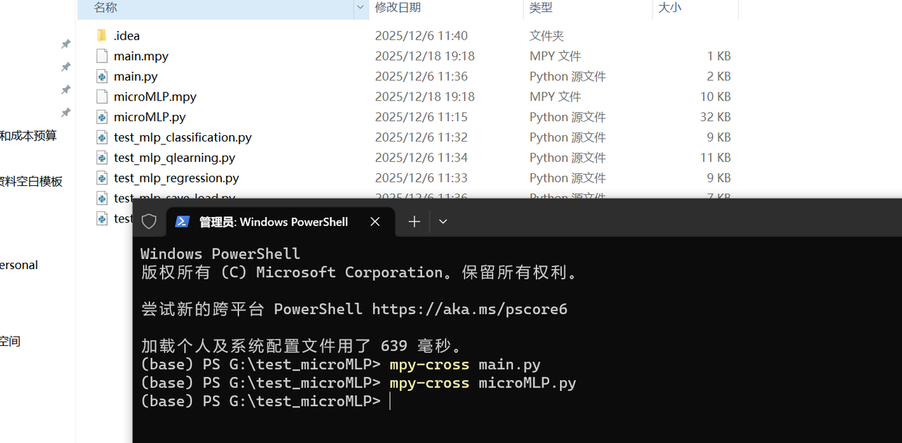
mpy-cross (MicroPython cross-compiler): the official cross-compile tool for MicroPython, which can pre-. py scripts into. mpy bytecode files on a personal computer (PC), then upload the. mpy files to a microcontroller for execution. Compared with dynamically compiling. py files on the device, pre-compiled. mpy bytecode has three advantages: it reduces the compile time on the device (especially when running a script for the first time, preventing the device from wasting computing power on compiling);. mpy files have a smaller size, saving flash space on the microcontroller;Bytecode loads and executes slightly faster than the original. py files.
The process of developing high-performance code consists of the following phases, which shall be executed in the listed order:
Identify the slowest parts in the code (profiling): This is the first and most critical step of optimization — if you optimize blindly, you might spend a huge amount of time optimizing code that is already fast, which is completely pointless. We use the timing feature of the utime module to measure the execution time of each function and locate the most time-consuming "performance bottleneck".
Improving the Efficiency of Python Code (Basic Optimization): Optimize the writing style of Python code without changing its execution logic (for example, using list comprehensions instead of for loops, using local variables instead of global variables — local variables are accessed faster in MicroPython, reducing unnecessary function calls, etc.). This step is the simplest and can solve most performance issues.
Use the native code emitter (intermediate optimization): If the performance is still insufficient, use MicroPython's @micropython. native decorator to compile the function into native machine code, which will significantly improve execution speed with almost no code modifications required.
Use the Viper code emitter (advanced optimization): If the native compile still doesn't deliver sufficient speed, use the @micropython. viper decorator, which enables the code to run at a speed close to that of C, but note that it comes with syntax restrictions (e. g., complex Python data structures cannot be used).
Use mpy-cross to compile into bytecode (pre-compilation optimization): If after the previous optimization, the loading time of the script on its first run is still long (especially for large scripts), use mpy-cross on a computer to pre-compile. py files into. mpy bytecode files, then upload them to the device. This step does not require modifying the code, only changes the file loading method, and can significantly reduce the compilation overhead on the device.
Hardware-Specific Optimization (Ultimate Optimization): This is the final step, which leverages the hardware peripherals of the microcontroller to replace software emulation — for example, using hardware DMA to transfer data and hardware timers to replace software-based delays. This is the ultimate solution for boosting performance.
3. Optimization Methods
3.1 Identify the Slowest Code
When identifying the slowest parts of the code, we can usually establish function groups recorded in ticks through the judicious use of timing utime. The code execution time can be measured in ms (milliseconds), us (microseconds), or CPU cycles.
The following allows you to add the @timed_function decorator to time any function or method:
import time

def timed_function(f, *args, **kwargs):
    myname = str(f).split(' ')[1]
    def new_func(*args, **kwargs):
        t = time.ticks_us()
        result = f(*args, **kwargs)
        delta = time.ticks_diff(time.ticks_us(), t)
        print('Function {} Time = {:6.3f}ms'.format(myname, delta/1000))
        return result
    return new_func
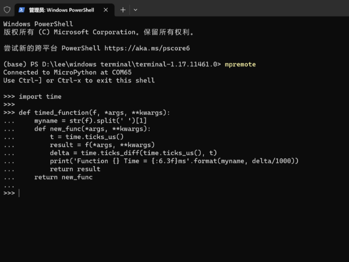
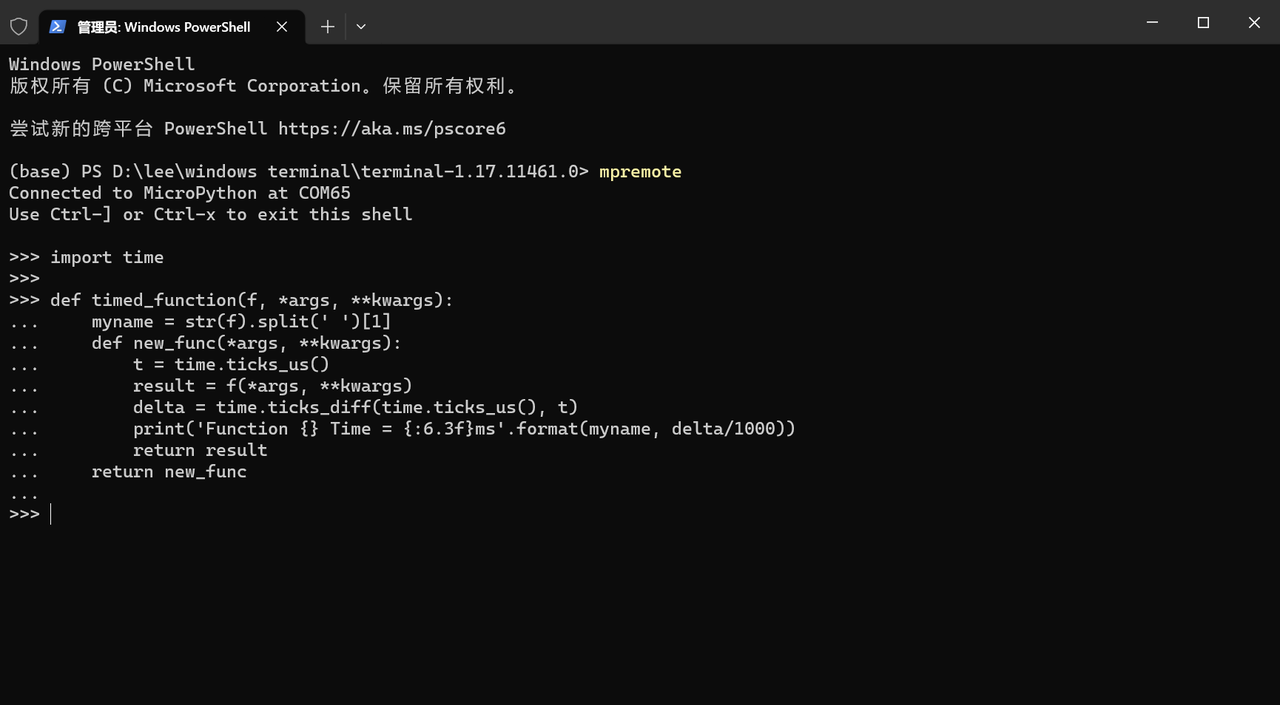
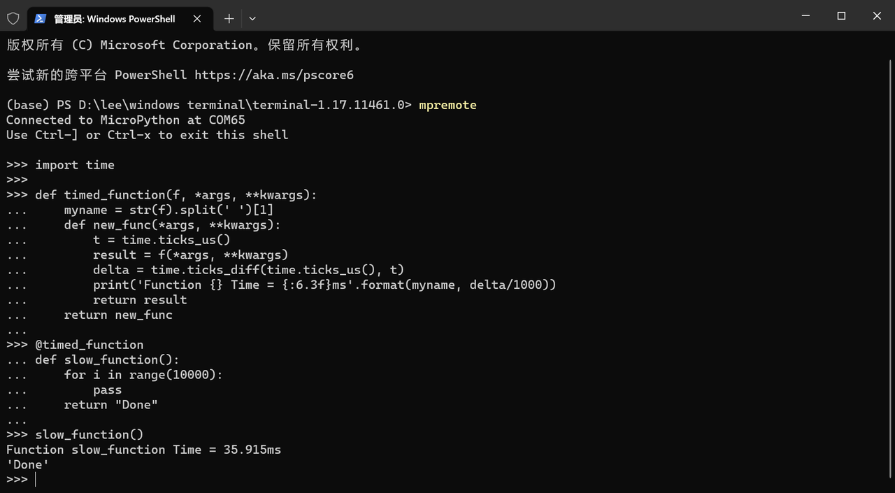
Here, we use the mpremote tool to connect to the Raspberry Pi Pico, copy the code above into the REPL, and press Enter to execute it (at this point, the decorator has been defined successfully):
Next, define a test function (to simulate time-consuming operations):
# 用@timed_function装饰器修饰测试函数
@timed_function
def slow_function():
    for i in range(10000):
        pass
    return "Done"
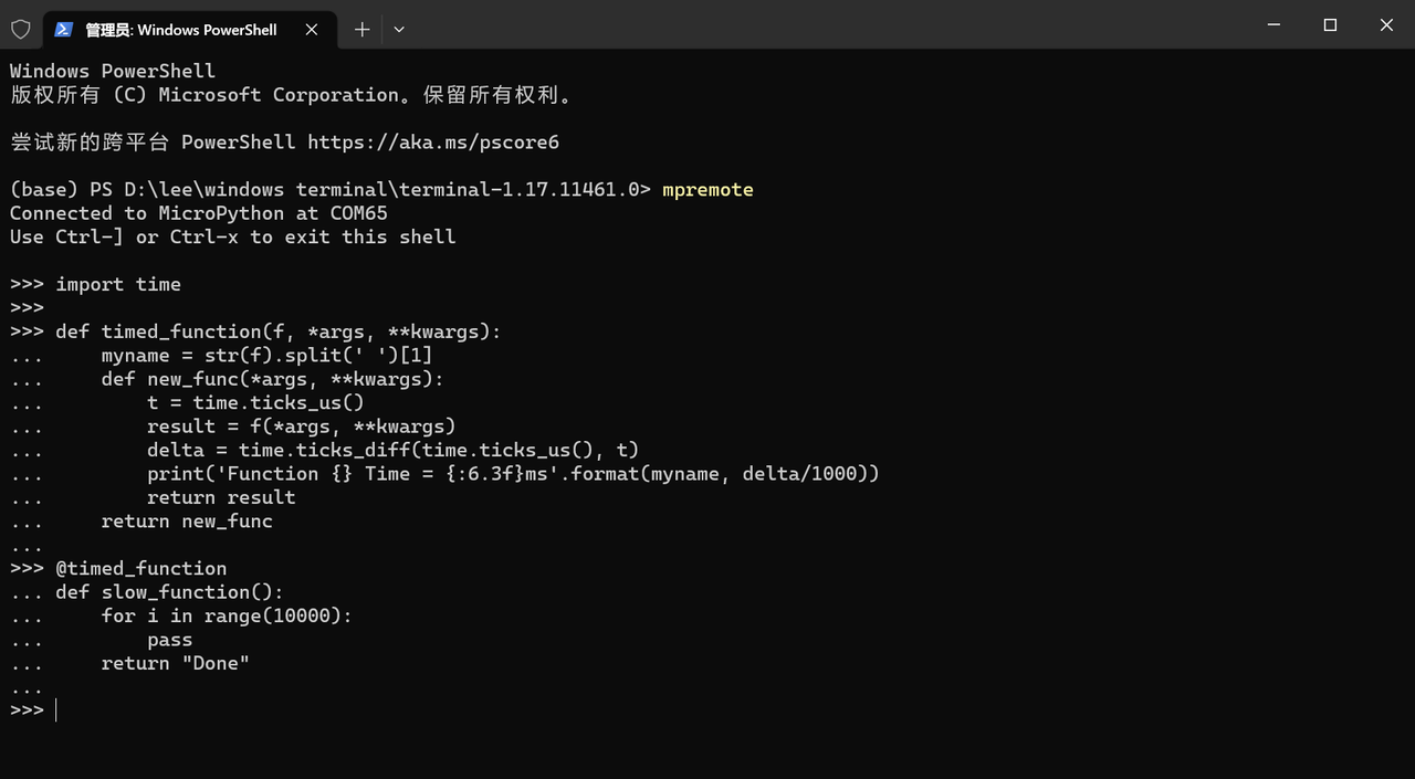
We will paste it into the REPL:
Then call the function and check the timing result:
slow_function()
We can see that the time consumption result of the function execution has been output:
3.2 Specific Measures for Performance optimization
3.2.1 Performance Bottlenecks and Core Fundamental Concepts of MicroPython
3.2.1.1 Core Basic Concepts
3.2.1.1.1 Variables and Constants
Here, first of all, we need to understand the difference between variables and constants, which is the foundation of programming, and the core difference between the two lies in when their values are determined:
Variables are dynamically assigned during runtime and their values can be modified. When MicroPython accesses a variable, it needs to look it up in the global or local dictionary, which incurs a small amount of overhead — this overhead will be amplified especially when variables are accessed frequently in loops.
# 变量,运行时存储在字典中
max_count = 10000
for i in range(max_count):
    # 每次循环都要查字典找max_count的值
    pass
Constants have values determined at compile time and cannot be modified. MicroPython provides the const () declaration (similar to C's #define), which directly replaces the identifier with the corresponding literal value when compiling bytecode, completely eliminating runtime dictionary lookup overhead.
from micropython import const
# 常量,编译时直接替换为10000
MAX_COUNT = const(10000)
for i in range(MAX_COUNT):
    # 循环中直接使用10000,无需查字典
    pass
3.2.1.1.2 Three Memory Partitions
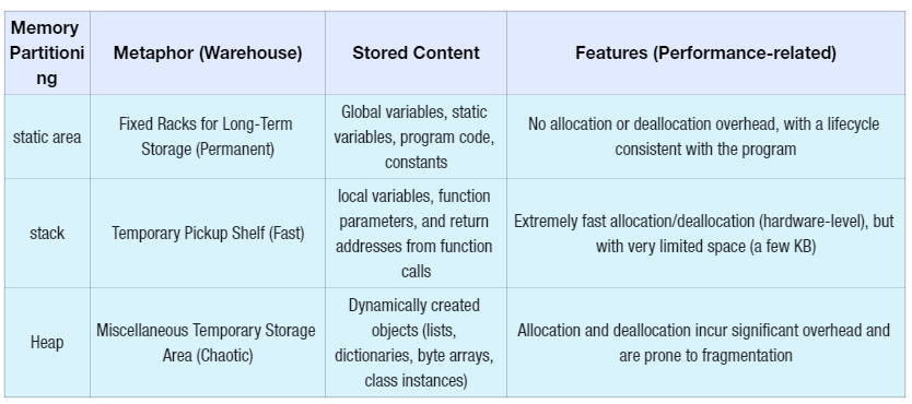
Embedded microcontrollers (such as the RP2040) have extremely limited memory resources (for example, only 264KB of RAM), and the object storage of MicroPython directly relies on memory partitions, where heap allocation and deallocation constitute the biggest performance bottleneck. We use the metaphor of "Warehouse Management" to understand the three partitions:
内存分区
比喻(仓库)
存储内容
特点(性能相关)
静态区
长期存储的固定货架(永久)
全局变量、static变量、程序代码、常量
无分配 / 回收开销,生命周期和程序一致
栈
临时取货的小货架(快速)
局部变量、函数参数、函数调用的返回地址
分配 / 释放极快(硬件级),但空间极小(几 KB)
堆
临时堆放的杂项区域(混乱)
动态创建的对象(列表、字典、字节数组、类实例)
分配 / 回收有显著开销,易产生碎片
For memory management in embedded development, we often face the following challenges:
Heap allocation requires traversing free memory blocks, which is time-consuming;
Objects that are no longer in use in the heap require garbage collection (GC) for cleanup, a process that blocks the program and takes several milliseconds, which is fatal in real-time scenarios;
The stack space is limited. If there are too many local variables or excessively deep function nesting, a stack overflow (immediate program crash) will be triggered.
3.2.1.1.3 Reference and Copy
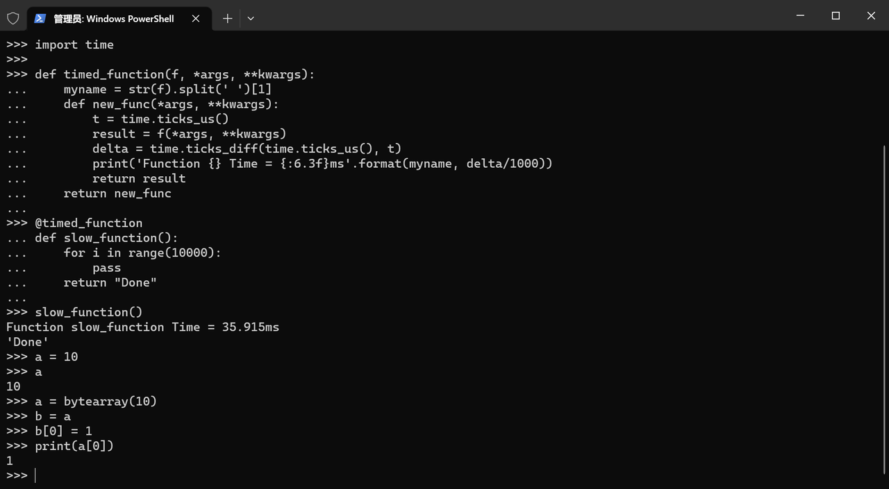
A reference, in essence, serves as the "house number"(analogous to a shortcut on a computer) of an object: what a variable stores is not the data itself, but the memory address of the data. Manipulating a reference does not copy the data, thus incurring extremely low overhead.
# 在堆上创建字节数组对象,a存储的是对象的地址(门牌号)
a = bytearray(10)
# b是a的引用,指向同一个对象,无新分配
b = a
# 操作b会改变a的内容,因为是同一个对象
b[0] = 1
# 输出:1
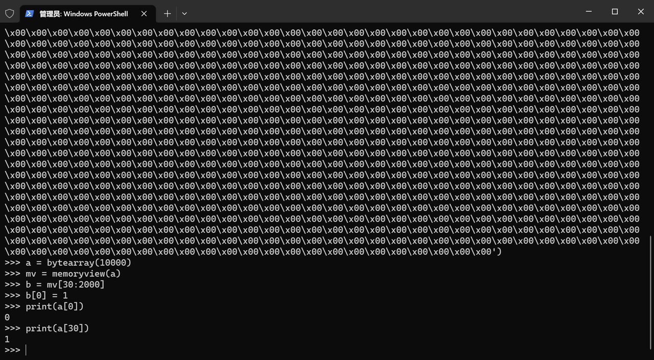
print(a[0])
In the terminal, the running result is as follows:
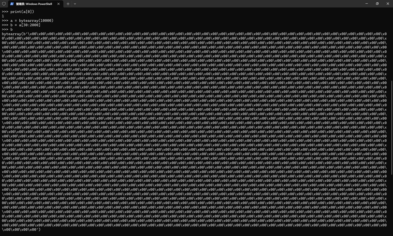
Then for copying (here referring to deep copy; we won’t go into detail about the difference between shallow copy and deep copy here), it replicates the entire data, creates a new object on the heap, and stores a new data set, which incurs extremely high overhead (especially for Big data):
# 大字节数组(堆上10KB)
a = bytearray(10000)
# 切片操作,创建新的字节数组(堆上~2KB),属于深拷贝
b = a[30:2000]
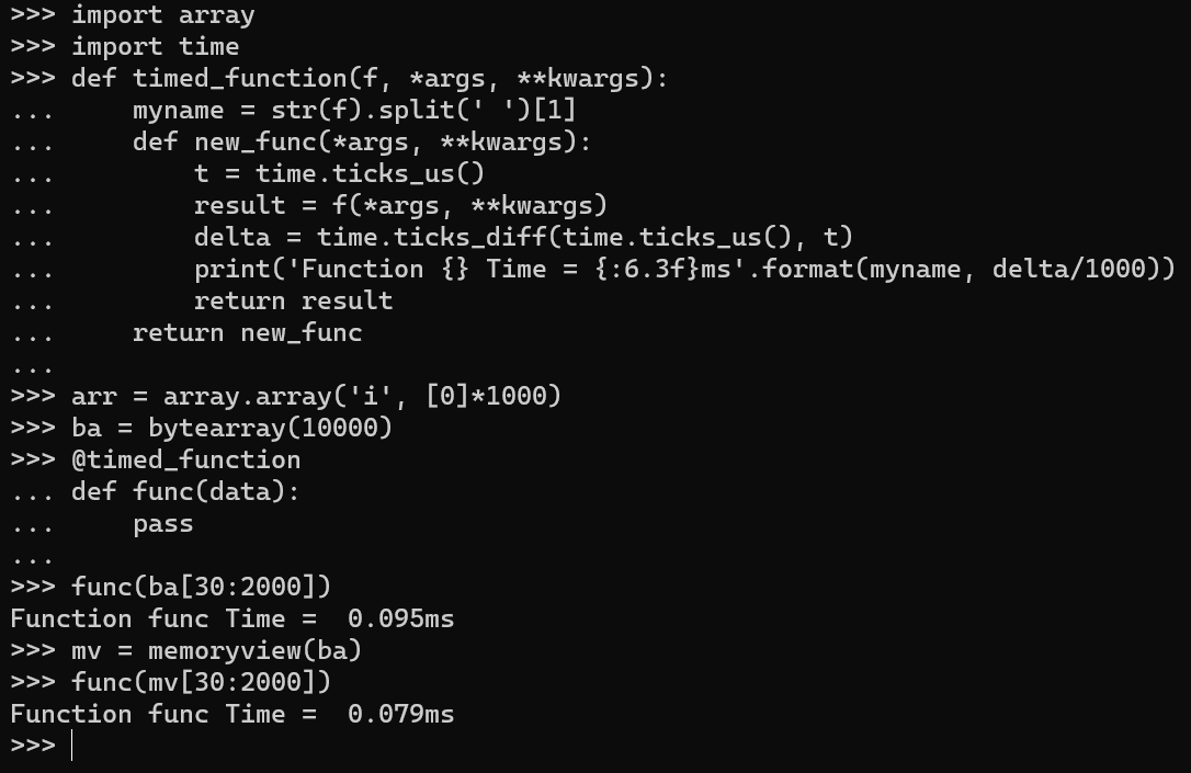
To avoid excessive heap allocation caused when copying large byte arrays, we can use memoryview, a shallow reference tool provided by MicroPython. Essentially, it acts as a "read/write access handle" for buffer objects such as bytearrays, arrays, and bytes. When slicing, it does not copy data but only passes the address, thus completely eliminating heap allocation.
It should be noted here that memoryview only supports buffer protocol objects (bytearray, array, bytes), and does not support lists (lists store object references rather than contiguous data).
Once you have mastered the above basics, you can then move on to understanding these advanced concepts of embedded MicroPython:
Garbage Collection (GC): MicroPython automatically cleans up objects in the heap that are no longer referenced, and this process will block the program. We can manually call gc. collect () to control the timing of cleanup to avoid triggering it in performance-critical sections.
native/viper code emitter: compile Python code into ARM-Thumb machine code (rather than bytecode), with an execution speed far exceeding that of interpreted execution (native runs twice as fast as bytecode, while viper adopts a more aggressive optimization strategy, supports pointer operations, and delivers performance close to that of the C language).
Direct register manipulation: Bypassing MicroPython's hardware abstraction layer (such as machine. Pin), directly reading and writing the register addresses of the chip to eliminate the overhead of method calls (suitable for high-frequency hardware operations).
mpy-cross: a MicroPython cross compiler that pre-compiles. py scripts into. mpy bytecode on a computer, so as to reduce the compile overhead on the device and speed up script loading.
3.2.1.2 Performance Bottlenecks of MicroPython
The performance bottlenecks of MicroPython mainly stem from three core aspects: the overhead of heap memory allocation and garbage collection (GC), the overhead of interpreted execution of Python bytecode, and inefficient operation/hardware operation methods.
Therefore, we can optimize from the following aspects:
Memory and Object Optimization (Highest Priority, Lowest Cost): Address the overhead issues of heap allocation and garbage collection (GC), which is the most common performance bottleneck in MicroPython embedded scenarios.
Code Execution Efficiency Optimization (Medium Priority): Improve the running speed of the code itself, with optimizations ranging from the bytecode level to the machine code level.
Operation and hardware optimization (lowest priority, suitable for performance-critical scenarios): It is the ultimate optimization approach that leverages hardware features to reduce inefficient operations/manipulations.
3.2.2 Memory and Object Optimization
The core of this type of optimization is to "avoid dynamically creating objects at runtime and reduce heap allocation as much as possible, thereby lowering the trigger frequency and time consumption of GC", which is the primary step for Performance optimization of embedded MicroPython.
3.2.2.1 Pre-allocated Memory and Fixed Object Size
The object is created only once (e. g., instantiated in the class constructor), and its size is not allowed to grow dynamically (e. g., list append, adding new Attribute–Value Pairs to a dictionary). Especially for buffers (such as buffers for serial communication), they shall be pre-allocated and to reuse.
We can use readinto () instead of read ()(read () allocates a new buffer each time, while readinto () reads data into an existing buffer).
Take the serial port buffer as an example:
from machine import UART, Pin

# 1. 预分配缓冲区(只创建一次,避免动态分配)
buf = bytearray(64)  # 预分配64字节的缓冲区

# 初始化UART
uart = UART(0, baudrate=9600, tx=Pin(0), rx=Pin(1))

# 2. 使用readinto()读入预分配的缓冲区(无新分配)
while True:
    if uart.any():
        # 数据读入buf,返回读取的字节数
        n = uart.readinto(buf)
        # 对比:uart.read(64) 会每次创建新的字节对象,触发堆分配
        print("recv data:", buf[:n])
3.2.2.2 Use arrays instead of lists + memoryview to avoid data copying
Lists store object references with non-contiguous memory, and dynamic growth will trigger heap allocation;array module (or bytearray) stores contiguous data of primitive types, delivering higher performance after pre-allocation; meanwhile, slicing operations (such as ba[30:2000]) will create data copies and trigger heap allocation; using memoryview enables direct passing of memory pointers with no copy overhead.
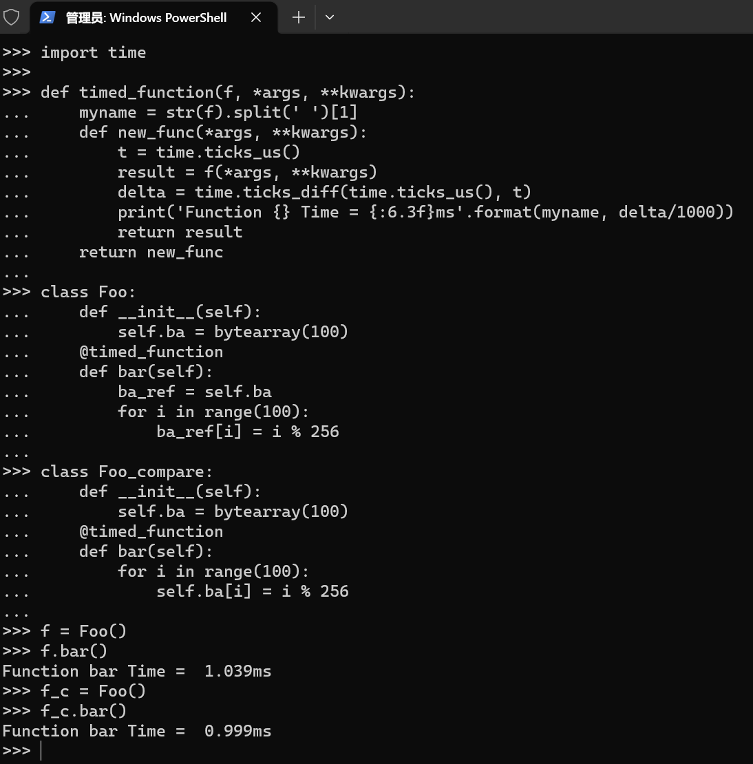
Cache frequently accessed objects (such as self. ba, obj_display. framebuffer) into local variables to avoid attribute lookups on every access — attribute lookups involve dictionary operations, which are time-consuming and may trigger memory allocation.
import time

def timed_function(f, *args, **kwargs):
    myname = str(f).split(' ')[1]
    def new_func(*args, **kwargs):
        t = time.ticks_us()
        result = f(*args, **kwargs)
        delta = time.ticks_diff(time.ticks_us(), t)
        print('Function {} Time = {:6.3f}ms'.format(myname, delta/1000))
        return result
    return new_func

class Foo:
    def __init__(self):
        self.ba = bytearray(100)
    @timed_function
    def bar(self):
        ba_ref = self.ba
        for i in range(100):
            ba_ref[i] = i % 256

class Foo_compare:
    def __init__(self):
        self.ba = bytearray(100)
    @timed_function
    def bar(self):
        for i in range(100):
            self.ba[i] = i % 256

# 测试
f = Foo()
f.bar()

f_c = Foo()
f_c.bar()
Click to run, and the terminal outputs the following:
3.2.2.4 Manual Garbage Collection Control
Call gc. collect () regularly to manually trigger GC, so as to prevent GC from being triggered randomly in performance-critical code segments (manual GC allows for timing control, and the time cost of frequent minor GCs is far lower than that of a single major GC).
import gc
import time

# 启用GC(默认启用,可手动关闭/开启)
gc.enable()
# 性能关键循环前,手动触发GC
# 提前清理内存,耗时约1ms
gc.collect()

# 性能关键代码段
start = time.ticks_us()
for i in range(10000):
    pass
end = time.ticks_us()

print(f"耗时:{utime.ticks_diff(end, start)/1000}ms")
# 定期在非关键段触发GC
# gc.collect()
3.2.3 Code Execution Efficiency Optimization
This type of optimization further improves the execution speed of the code on the basis of memory optimization, and conducts optimization from the bytecode level to the machine code level.
3.2.3.1 Declare constants using const ()
const () replaces identifiers with numerical values (completed at compile time), avoiding runtime dictionary lookups, and delivers particularly significant optimization effects for constants used in loops.
from micropython import const
import time

# 声明常量(编译时替换为数值)
MAX_COUNT = const(100000)
# 二进制常量也支持
PIN_BIT = const(1 << 2)

MAX_COUNT_NOT_USE_CONST = 100000

def timed_function(f, *args, **kwargs):
    myname = str(f).split(' ')[1]
    def new_func(*args, **kwargs):
        t = time.ticks_us()
        result = f(*args, **kwargs)
        delta = time.ticks_diff(time.ticks_us(), t)
        print('Function {} Time = {:6.3f}ms'.format(myname, delta/1000))
        return result
    return new_func

@timed_function
def use_const():
    total = 0
    for i in range(MAX_COUNT):
        total += i
    return total

# 对比:不用const(),每次访问都会查字典,耗时更长
@timed_function
def no_const():
    global MAX_COUNT_NOT_USE_CONST
    total = 0
    for i in range(MAX_COUNT_NOT_USE_CONST):
        total += i
    return total

result1 = use_const()
result2 = no_const()
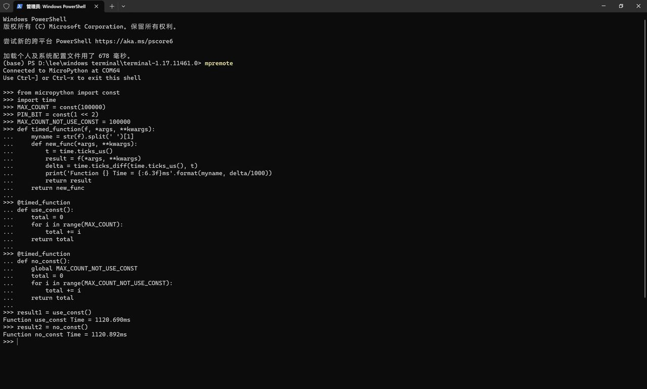
The running result in the terminal is as follows:
We can see that the running time of the two is actually almost the same, because in the REPL, the code is executed in an interpreted manner, while const 's real advantage only becomes obvious in pre-compiled bytecode.
3.2.3.2 mpy-cross compile bytecode
Use mpy-cross on a computer to pre- compile. py scripts into. mpy bytecode, then upload it to the device.
We can use the pip command to install the mpy-cross tool:
Then, use the following command to compile MicroPythonpy files into mpy files:
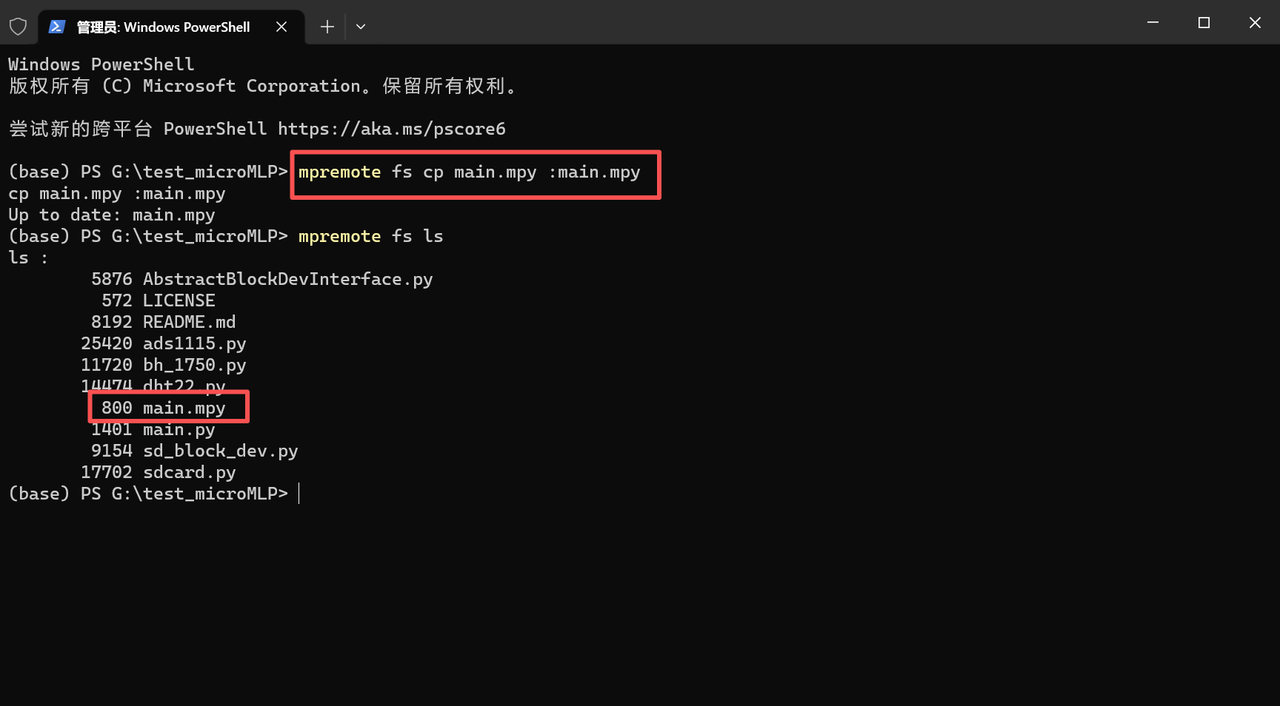
We can see that the compiled mpy file is smaller. Then just use the mpremote tool to transfer it to the device side.
3.2.3.3 Using a Code Emitter
When MicroPython compiles code, it processes each function individually (classes are functions, as are lambdas and list comprehensions). Functions emerge from the parsing phase and then enter the compiler, which passes the Python function three times:
In the first phase, the compiler collects information about variables and their scopes (local or global), and determines the emitter type by looking for special types of function decorators;
In the second phase, it calculates the stack usage and code offsets;
In the third stage, the code is transmitted by the required transmitter.
Currently, there are four types of code transmitters:
Bytecode Emitter: By default, functions use the bytecode emitter, and the generated bytecode runs on MicroPython's built-in virtual machine. The virtual machine is extremely straightforward: it decodes each bytecode (along with its parameters, if any) and invokes the corresponding C runtime function;
native code emitter: The native code emitter takes each bytecode and converts it into equivalent ARM-Thumb machine code. Functions of this type use the standard C stack to store local variables and directly call C runtime functions; however, note that they cannot be used in context managers (with statements) and generators, and if raise is used, arguments must be provided;
Viper Code Emitter: compile into optimized machine code, supports pointer operations, and its speed is close to that of C language (with more compatibility restrictions).
Inline Assembler: Not to be discussed for now, please refer to the link http://www.86x.org/en/latet/reference/asm_thumb2_index.html .
3.2.3.3.1 native code emitter
The native code emitter takes each bytecode and converts it into equivalent ARM-Thumb machine code. Such functions use the ordinary C stack to store local variables and directly call C runtime functions.
The native code emitter is invoked via a function decorator:
The current implementation of the native code emitter has certain limitations:
Context managers (the `with` statement) are not supported
Generators are not supported
If raise is used, parameters must be provided
The tradeoff for improved performance (roughly twice that of bytecode) is an increase in the size of the compiled code.
3.2.3.3.2 Viper Code Transmitter
The optimizations discussed above involve standard-compliant Python code. The Viper code emitter is not fully compatible. It supports special Viper native data types in pursuit of performance. Integer processing is non-compliant because it uses machine words: arithmetic on 32-bit hardware is performed modulo 2**32.
The Viper code emitter generates ARM-Thumb machine code for each bytecode and further optimizes certain operations, such as integer arithmetic. For the addition of two integers, the Viper emitter does not call the C runtime function rt_binary_op, but instead emits the machine instruction "adds" to directly add the two numbers. This is significantly faster than calling rt_binary_op. It is invoked using a decorator:
Viper supports its own set of types, namely int, uint (unsigned integer), ptr, ptr8, ptr16 and ptr32:
ptr: pointer to the object
ptr8 points to a byte
ptr16 points to a 16-bit halfword
ptr32 points to a 32-bit machine word
Here, we will test the integer accumulation with heavy computational load:
import time
import micropython

def timed_function(name):
    def decorator(f):
        def new_func(*args, **kwargs):
            t = time.ticks_us()
            result = f(*args, **kwargs)
            delta = time.ticks_diff(time.ticks_us(), t)
            print('Function {} Time = {:6.3f}ms'.format(name, delta/1000))
            return result
        return new_func
    return decorator

# 普通Python函数:100万次累加(手动指定函数名'normal_add_loop')
@timed_function('normal_add_loop')
def normal_add_loop(n: int) -> int:
    total = 0
    for i in range(n):
        total += i * 2 + 5
    return total

# Viper优化函数:相同计算量(手动指定函数名'viper_add_loop')
@timed_function('viper_add_loop')
@micropython.viper
def viper_add_loop(n: int) -> int:
    total = 0
    for i in range(n):
        total += i * 2 + 5
    return total

# 调用测试(100万次运算,正常计时输出)
normal_add_loop(1000000)
viper_add_loop(1000000)
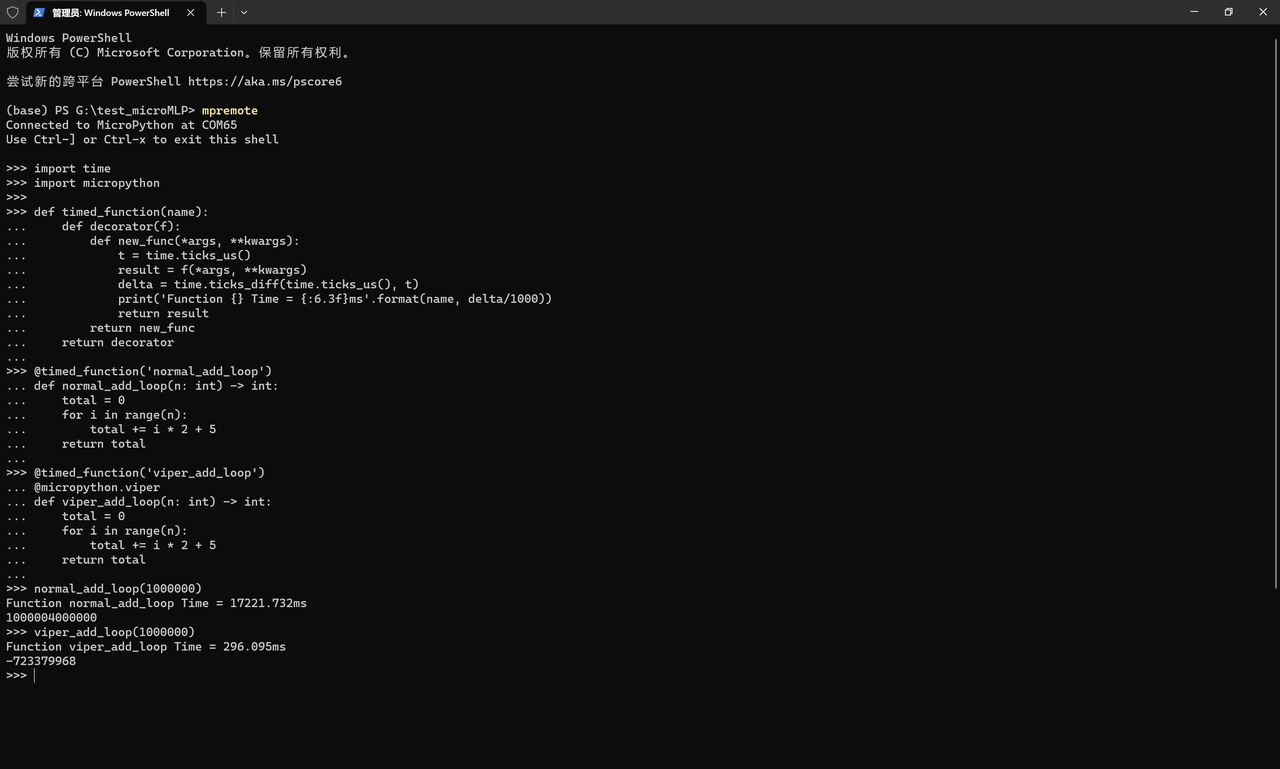
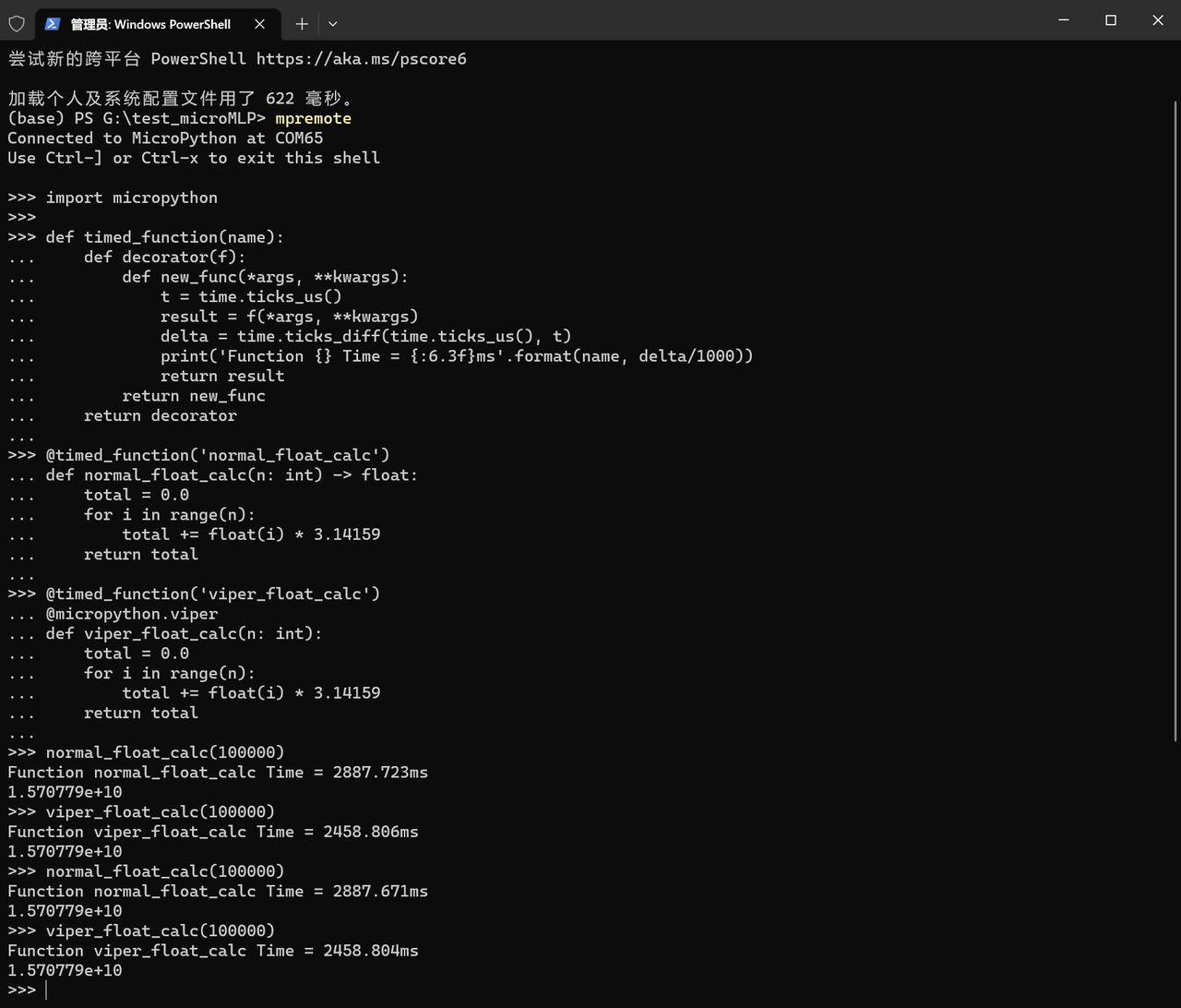
Both functions perform exactly the same 1 million integer operations (i*2+ 5 accumulation), but normal_add_loop is purely interpreted for execution, while viper_add_loop is directly executed as machine code. The terminal running results are as follows:
We conducted tests on the Raspberry Pi Pico, where the time consumption of normal_add_loop is dozens of times that of viper_add_loop.
Viper has two key limitations:
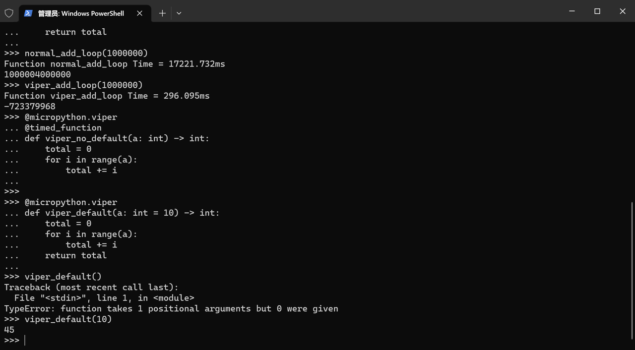
Default parameters are not allowed: function parameters cannot be assigned a: int = 10 as a default value, otherwise an error will be thrown.
Floating-point operations are usable but unoptimized: The time consumption of floating-point calculation is almost identical to that of an ordinary Python function, as Viper does not generate optimized machine code for floating-point operations.
import micropython
# 错误示例(REPL运行会报错:Viper does not support default arguments)
# @micropython.viper
# def viper_default(a: int = 10) -> int:
#     total = 0
#     for i in range(a):
#         total += i
#     return total

# 正确示例(无默认参数,100万次运算,计时)
@micropython.viper
@timed_function
def viper_no_default(a: int) -> int:
    total = 0
    for i in range(a):
        total += i
    return total

# 调用测试
viper_no_default(1000000)
The running results are as follows:
Let's test the floating-point operations of the function compiled by Viper and ordinary functions again:
import micropython

def timed_function(name):
    def decorator(f):
        def new_func(*args, **kwargs):
            t = time.ticks_us()
            result = f(*args, **kwargs)
            delta = time.ticks_diff(time.ticks_us(), t)
            print('Function {} Time = {:6.3f}ms'.format(name, delta/1000))
            return result
        return new_func
    return decorator

# 普通函数:10万次浮点乘法累加
@timed_function('normal_float_calc')
def normal_float_calc(n: int) -> float:
    total = 0.0
    for i in range(n):
        total += float(i) * 3.14159
    return total

# Viper函数:相同的10万次浮点运算(无优化)
@timed_function('viper_float_calc')
@micropython.viper
def viper_float_calc(n: int):
    total = 0.0
    for i in range(n):
        total += float(i) * 3.14159
    return total

# 调用测试(计时结果几乎一致)
normal_float_calc(100000)
viper_float_calc(100000)
The running results are as follows:
The pointer types in Viper (ptr8/ptr16/ptr32) are used to directly access contiguous memory (such as bytearray) without boundary checking, and support single-element access via subscripts (slicing is not supported). A key optimization technique is: to place the operation of converting an object to a pointer at the beginning of the function rather than inside a loop, as the conversion takes several microseconds, which will be amplified in large loops.
The advantages of pointers are particularly prominent in large array traversal scenarios, being far faster than array access in standard Python.
import micropython

def timed_function(name):
    def decorator(f):
        def new_func(*args, **kwargs):
            t = time.ticks_us()
            result = f(*args, **kwargs)
            delta = time.ticks_diff(time.ticks_us(), t)
            print('Function {} Time = {:6.3f}ms'.format(name, delta/1000))
            return result
        return new_func
    return decorator

# 准备1万长度的bytearray(大数组)
ba = bytearray(10000)
for i in range(10000):
    ba[i] = i % 256

# 普通函数:遍历10万bytearray,累加值
@timed_function('normal_bytearray_access')
def normal_bytearray_access(ba: bytearray) -> int:
    total = 0
    for i in range(10000):
        total += ba[i]
    return total

# Viper函数:ptr8指针访问,累加值(转换放在开头)
@timed_function('viper_ptr8_access')
@micropython.viper
def viper_ptr8_access(ba) -> int:
    buf = ptr8(ba)
    total = 0
    for i in range(10000):
        total += buf[i]
    return total

# 调用测试(指针访问速度远超普通访问)
normal_bytearray_access(ba)
viper_ptr8_access(ba)
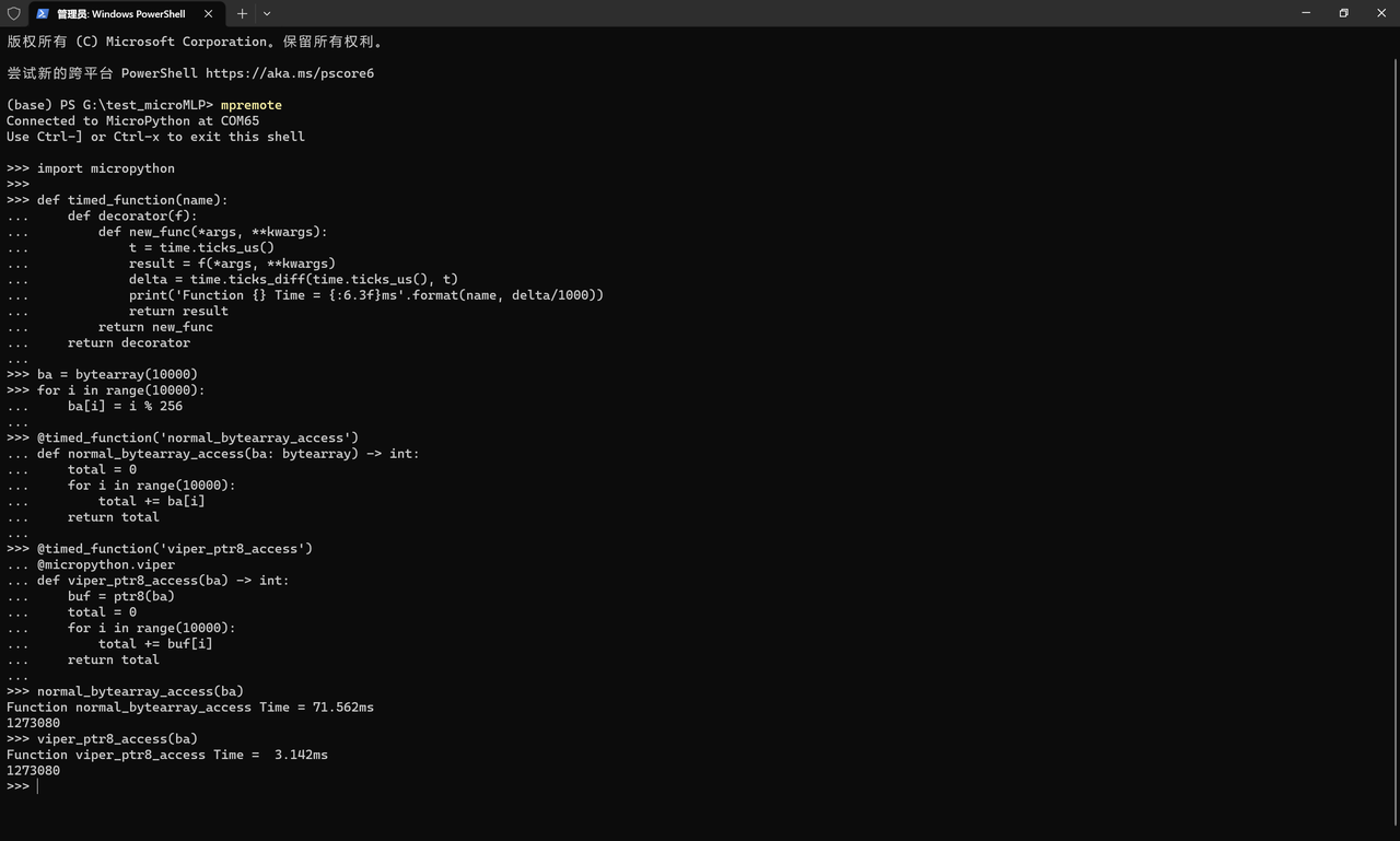
The terminal output is as follows:
viper_ptr8_access takes only one-thirtieth of the time of normal_bytearray_access in a regular function requires steps such as Python's boundary check and object attribute lookup; the ba[i]in a regular function requires steps such as Python's boundary check and object attribute lookup; the buf[i]in Viper directly calculates the memory address and accesses the byte, with no additional overhead.
Next, let's compare the difference between performing the operation of converting an object to a pointer inside a loop versus doing it at the beginning:
import micropython

def timed_function(name):
    def decorator(f):
        def new_func(*args, **kwargs):
            t = time.ticks_us()
            result = f(*args, **kwargs)
            delta = time.ticks_diff(time.ticks_us(), t)
            print('Function {} Time = {:6.3f}ms'.format(name, delta/1000))
            return result
        return new_func
    return decorator

# 准备1万长度的bytearray(大数组)
ba = bytearray(10000)
for i in range(10000):
    ba[i] = i % 256

# Viper函数:循环内重复转换ptr8(低效)
@timed_function('viper_bad_convert')
@micropython.viper
def viper_bad_convert(ba) -> int:
    total = 0
    for i in range(10000):
        buf = ptr8(ba)
        total += buf[i]
    return total

# Viper函数:开头一次性转换ptr8(高效)
@timed_function('viper_good_convert')
@micropython.viper
def viper_good_convert(ba) -> int:
    buf = ptr8(ba)
    total = 0
    for i in range(10000):
        total += buf[i]
    return total

# 调用测试(低效版耗时远高于高效版)
viper_bad_convert(ba)
viper_good_convert(ba)
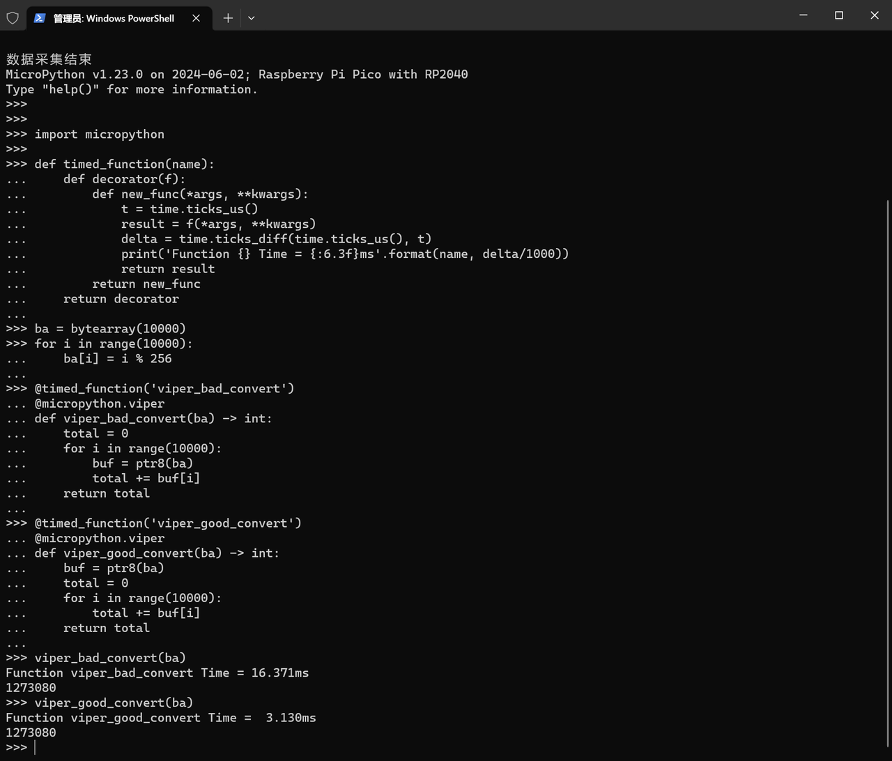
The running results are as follows:
viper_bad_convert performs a type conversion on ptr8 (ba) in each of 1 million loops (each conversion takes a few microseconds, resulting in significant cumulative time);viper_good_convert performs the conversion only once at the start, eliminating redundant overhead.
Viper's integers operate at the machine word level, with arithmetic operations executed modulo 2**32 on 32-bit hardware (truncation occurs upon overflow), which is a trade-off of compatibility for performance, and this characteristic becomes more pronounced under heavy computational loads.
3.2.4 Operation and hardware Optimization
3.2.4.1 Replace Floating-Point Operations with Integer Operations
Chips without an FPU (floating-point coprocessor) execute floating-point operations extremely slowly, so integer operations are used for performance-critical parts, while non-critical parts are converted to floating-point numbers.
from machine import ADC, Pin
import array

def timed_function(f, *args, **kwargs):
    myname = str(f).split(' ')[1]
    def new_func(*args, **kwargs):
        t = time.ticks_us()
        result = f(*args, **kwargs)
        delta = time.ticks_diff(time.ticks_us(), t)
        print('Function {} Time = {:6.3f}ms'.format(myname, delta/1000))
        return result
    return new_func

# 1. 纯整数运算:预分配数组+ADC读数(无浮点)
# 预分配100个int型元素的数组(连续内存,无动态分配)
# 纯整数运算:读取16位整数ADC值
@timed_function
def adc_read_integer():
    adc_data = array.array('i', [0]*100)
    adc = ADC(Pin(26))

    for i in range(100):
        adc_data[i] = adc.read_u16()
    return adc_data

# 2. 包含浮点运算:整数读数+浮点转换(电压计算)
# 第一步:整数读数(和上面一致)
# 第二步:浮点运算转换为电压(读数/65535*3.3)
@timed_function
def adc_read_float():
    adc_data = array.array('i', [0]*100)
    adc = ADC(Pin(26))

    for i in range(100):
        adc_data[i] = adc.read_u16()

    voltage_data = [x/65535*3.3 for x in adc_data]
    return voltage_data

# 执行测试,对比耗时
print("=== ADC读数性能对比 ===")
integer_data = adc_read_integer()
float_data = adc_read_float()

# 打印前5个电压值(验证功能)
print("\n前5个电压值:", float_data[:5])
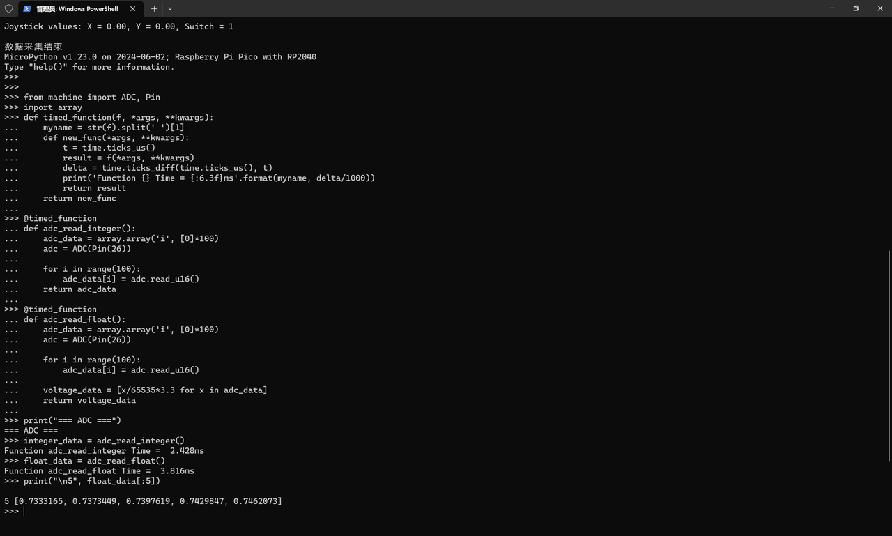
Terminal running:
We can see that the time consumed by floating-point operations is longer than that of pure integer operations.
3.2.4.2 Direct Register Read/Write
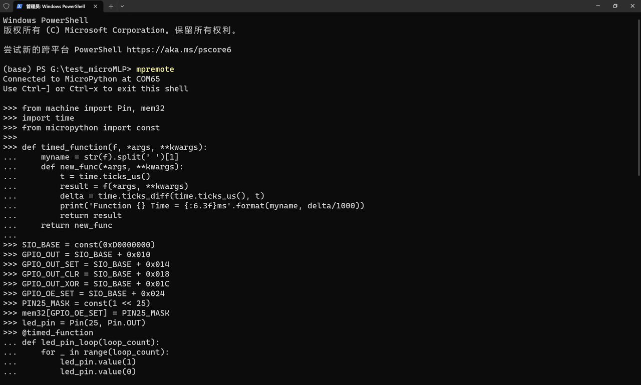
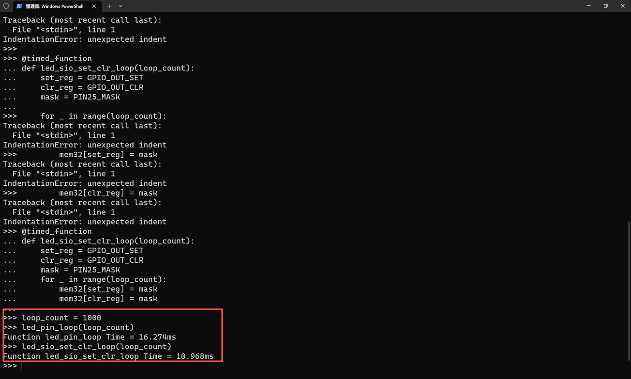
Bypass MicroPython's hardware abstraction layer to directly read and write chip registers, eliminating the overhead of method calls (e. g. fast LED blinking, high-frequency GPIO operations).
As can be seen, in the SIO loop function, GPIO_OUT_SET, GPIO_OUT_CLR, and PIN25_MASK are cached into local variables, which reduces the overhead of global variable lookup and makes the performance advantage of SIO more prominent.
3.2.4.3 DMA-related Operations
In scenarios involving computation and hardware data interaction (such as batch ADC Data Acquisition, high-frequency GPIO signal output, and sensor data stream reading), the CPU often needs to spend a large amount of time executing data transfer operations (such as reading data from peripheral registers to memory and writing computation results to GPIO registers), which preempts the resources required for computation.The DMA (Direct Memory Access) controller of the RP2040 can independently complete bulk data transfers between memory and peripherals/registers without CPU intervention, and its core optimization value lies in: freeing the CPU from tedious data transfer tasks so that it can focus on core computing logic.
From the perspective of development and performance, MicroPython only provides basic support for RP2040 DMA, capable of simple bulk data transmission only. In contrast, C language (Pico SDK) allows full configuration of the DMA's transmission mode, trigger conditions and data processing rules. Combined with direct register operations, it enables seamless optimization of arithmetic operations and hardware data interaction, making it the optimal choice for high-throughput and low-latency scenarios.